Introduction

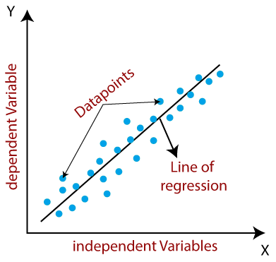
Linear regression is a statistical modeling technique used to analyze the relationship between a dependent variable and one or more independent variables. It assumes a linear relationship between these variables and aims to find the best-fitting line that accurately represents the data. This method is fundamental in data analysis and predictive modeling due to its straightforward approach to modeling relationships. Linear regression operates under the assumption that changes in the dependent variable are proportional to changes in the independent variable(s).

Classification and Regression

Classification predictive modeling problems are different from regression predictive modeling problems.

• Classification is the task of predicting a discrete class label.
• Regression is the task of predicting a continuous quantity.
  

There is some overlap between the algorithms for classification and regression; for example:

• A classification algorithm may predict a continuous value, but the continuous value is in the form of a probability for a class label.
• A regression algorithm may predict a discrete value, but the discrete value in the form of an integer quantity.
  

Some algorithms can be used for both classification and regression with small modifications, such as decision trees and artificial neural networks. Some algorithms cannot, or cannot easily be used for both problem types, such as linear regression for regression predictive modeling and logistic regression for classification predictive modeling.

Importantly, the way that we evaluate classification and regression predictions varies and does not overlap, for example:

• Classification predictions can be evaluated using accuracy, whereas regression predictions cannot.
• Regression predictions can be evaluated using root mean squared error, whereas classification predictions cannot.

Some common types of Linear Regression

• Simple Linear Regression : Involves a single independent variable predicting a dependent variable.
• Multiple Linear regression : Involves multiple independent variables predicting a dependent variable.

The main objective is to identify the best-fitting line, which is achieved by minimizing the differences between observed data points and their predicted values on this line. The characteristics of this line, defined by its slope and y-intercept, indicate the direction and starting point of the relationship, respectively.

Mathematically, we can represent a linear regression as: y=b₀+b₁x where:

• y : is the dependent variable or the variable we want to predict,
• x : is the independent variable or the variable used to predict y,
• b₀ : is the y-intercept, representing the value of y when x is zero,

$b_0=\frac{(\sum y)(\sum x^2)-(\sum x)(\sum xy)}{n(\sum x^2)-{(\sum x)}^2}$

• b₁ : is the slope or coefficient, indicating the change in y for a unit change in x, $b_1=\frac{n(\sum xy)-(\sum x)(\sum y)}{n(\sum x^2)-{(\sum x)}^2}$

• n : is the total no. of observations.

Example:

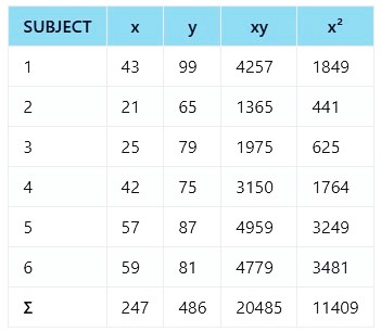
Let's consider a dataset that shows the relationship between the number of Age (x) and the corresponding Fever level (y) of 6 students. We want to build a linear regression model to predict the Fever level based on the age.

Step 1: Calculate xy, x² and Σ :

Step 2: Calculate b₀ and b₁:

Given data:

• n = 6 (number of observations)
• Σx = 247 (sum of x values)
• Σy = 486 (sum of y values)
• Σxy = 20485 (sum of x * y)
• Σx² = 11409 (sum of Σx²)

Find b₀:

$b_0=\frac{(\sum y)(\sum x^2)-(\sum x)(\sum xy)}{n(\sum x^2)-{(\sum x)}^2}$ $=\frac{486\ast 11409-247\ast 20485}{6\ast 11409-{(247)}^2}\backslash$ $=65.14\dots \dots \dots \dots \dots \left(1\right)$

Find b₁:

$b_1=\frac{n(\sum xy)-(\sum x)(\sum y)}{n(\sum x^2)-{(\sum x)}^2}$ $=\frac{6\ast 20485-247\ast 486}{6\ast 11409-{(247)}^2}$ $=0.38\dots \dots \dots \dots \dots \left(2\right)$

Step 3: Insert the values into the equation:

using values from (1) and (2)

$\mathrm{y\text{'}}=b_0+b_{1}x$

$\mathrm{y\text{'}}=65.14+(0.38\ast \mathrm{x})$

Step 4: Prediction - the value of y for the given value of x = 55:

$\mathrm{y\text{'}}=65.14+(0.38\ast 55)$

$\mathrm{y\text{'}}=86.04$

Output :

The linear regression equation for the given data is:

$\mathrm{y\text{'}}=65.14+(0.38\ast \mathrm{x})$

Prediction for x = 55:

$\mathrm{y\text{'}}=86.04$

Applications of Linear Regression:

• Economics : Predicting consumer demand, analyzing price elasticity, and estimating market trends.
• Finance : Modeling stock returns, predicting asset prices, and assessing risk factors.
• Healthcare : Analyzing the relationship between medical variables, predicting patient outcomes.
• Social Sciences : Investigating the impact of variables on social phenomena, analyzing survey data.
• Marketing : Determining the effectiveness of advertising campaigns, forecasting sales.

Advantages of Linear Regression:

• Simple and easy to understand.
• Provides insights into the relationship between variables.
• Can be used for both prediction and inference.
• Computationally efficient for large datasets.
• Provides measures of uncertainty and statistical significance.

Disadvantages of Linear Regression:

• Assumes a linear relationship between variables, which may not always hold.
• Sensitive to outliers and influential observations.
• Cannot capture complex nonlinear relationships between variables.
• Requires the absence of multicollinearity (high correlation) among independent variables.
• May be affected by heteroscedasticity (unequal variances of errors).