Introduction

Hierarchical clustering is an unsupervised machine learning algorithm used to group unlabeled datasets into clusters in a hierarchical manner. It is also known as hierarchical cluster analysis or HCA. This clustering method builds a tree-like structure, known as a dendrogram, to represent the relationships and hierarchy among the data points. Sometimes, the results of K-means clustering and hierarchical clustering may appear similar, but they differ based on their working mechanisms. Unlike the K-Means algorithm, there is no requirement to predetermine the number of clusters.

Basically, there are two types of hierarchical Clustering:

1. Agglomerative Clustering
2. Divisive Clustering

Agglomerative Clustering:

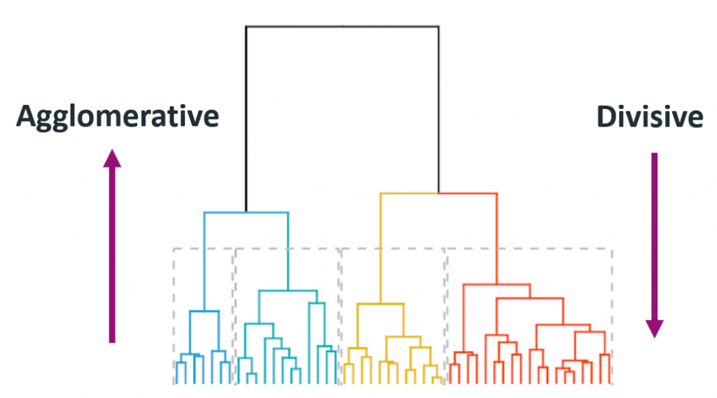
It starts with each data point as its own cluster and then iteratively merges the closest pairs of clusters until all data points belong to a single cluster. The merging process continues based on a chosen linkage criterion, such as complete linkage, single linkage, or average linkage. This approach is also known as the 'bottom-up' approach or hierarchical agglomerative clustering (HAC).

• Single Linkage: For two clusters R and S, the single linkage returns the minimum distance between two points i and j such that i belongs to R and j belongs to S.

  
  
  

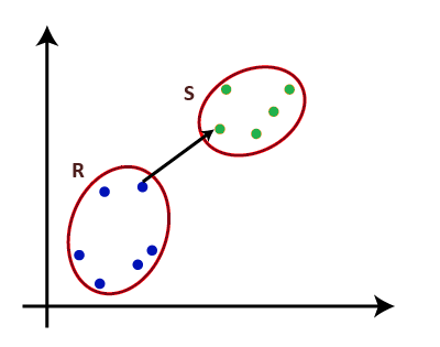
• Complete Linkage: For two clusters R and S, the complete linkage returns the maximum distance between two points i and j such that i belongs to R and j belongs to S.

  
  
  

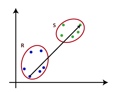
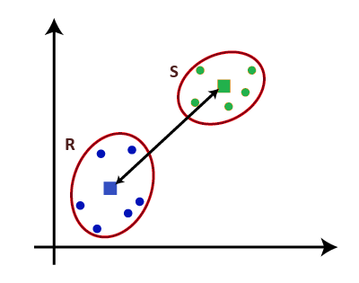
• Average Linkage: For two clusters R and S, first for the distance between any data-point i in R and any data-point j in S and then the arithmetic mean of these distances are calculated. Average Linkage returns this value of the arithmetic mean.

         where,
         n_R – Number of data-points in R
         n_S – Number of data-points in S

The algorithm progresses, forming a dendrogram that visually represents the hierarchy of the clusters. Some of the applications in which Agglomerative Clustering is used : Image segmentation, Customer segmentation, Social network analysis, Document clustering, Genetics, genomics, etc., and many more.

Dendrogram:

The dendrogram is a tree-like structure mainly used to store each step as a memory that the hierarchical clustering (HC) algorithm performs.

• Leaf: Individual
• Root: One cluster

A cluster at level 1, is the merger of its child cluster at level i+1.

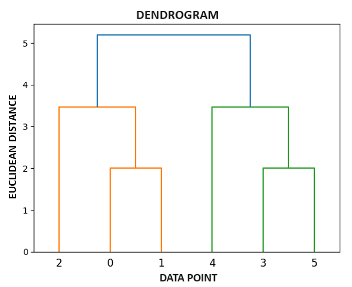
In the dendrogram plot, the Y-axis shows the Euclidean distances between the data points, while the X-axis displays all the data points of the given dataset.

Steps to perform Agglomerative Clustering:

1. Data Preparation: Collect and preprocess your dataset. Ensure that the data is in a suitable format.
2. Distance Matrix Calculation: Calculate the pairwise distances between all data points using an appropriate distance metric (e.g., Euclidean distance, Manhattan distance, etc.).
3. Initial Clustering: Treat each data point as a singleton cluster, forming an initial set of clusters.
4. Cluster Similarity Measurement: Measure the similarity between clusters based on the pairwise distances calculated. Common linkage criteria include: single linkage, complete linkage & average linkage.
5. Merge Closest Clusters: Iteratively merge the two clusters with the smallest distance according to the chosen linkage criterion. Update the distance matrix accordingly.
6. Dendrogram Construction: Build a dendrogram to visually represent the hierarchy of cluster relationships. The height of the dendrogram represents the distance at which clusters are merged.
7. Continue Merging: Repeat the merging process until all data points belong to a single cluster. The dendrogram will provide insights into the hierarchy and structure of the data.

Divisive Clustering:

Divisive clustering is a technique that starts with all data points in a single cluster and recursively splits the clusters into smaller sub-clusters based on their dissimilarity. It is also known as 'top-down' clustering. The process begins with all data points in a single cluster and then recursively splits the clusters into smaller sub-clusters based on their dissimilarity.
Some of the applications in which Divisive Clustering is used : Market segmentation, Anomaly detection, Biological classification, Natural language processing, etc.

Steps to perform Divisive Clustering:

1. Initialization: All data points form a single cluster.
2. Dissimilarity Calculation: Calculate dissimilarity between data points. For simplicity, let's use Euclidean distance.
3. Divide the Cluster: Identify the pair of data points with the highest dissimilarity.
4. Recursive Process: Treat each sub-cluster as a new cluster and repeat the process.
5. Result: The process continues recursively until each data point forms its own singleton cluster.

Steps to perform Divisive Clustering using Minimum Spanning Tree:

1. Graph Construction: Represent your dataset as a complete graph, where each data point is a node, and the edge weights are calculated based on dissimilarity (inverse similarity).
2. Minimum Spanning Tree: Use an algorithm to find the Minimum Spanning Tree (MST) of the graph. Kruskal's or Prim's algorithm are common choices.
3. Divisive Clustering: Consider the MST as a hierarchy. The initial cluster is the entire dataset. The first division could be achieved by cutting the MST at the edge with the highest weight.
4. Recursive Process: Continue recursively, treating each connected component of the graph after a cut as a new cluster, and apply the divisive clustering approach within each sub-cluster.

This conceptual integration can provide a hierarchical approach similar to divisive clustering, but it's essential to note that the conventional divisive clustering process doesn't explicitly involve MST.

Applications of Hierarchical Clustering:

• Biology: Phylogenetic tree construction based on genetic similarity.
• Marketing: Customer segmentation based on purchasing behavior.
• Image Segmentation: Grouping similar regions in an image.
• Document Clustering: Organizing documents based on topic similarity.

Advantages of Hierarchical Clustering:

• Interpretability: Hierarchical clustering produces dendrograms that visually represent the relationships between clusters. This makes it easy to interpret and understand the hierarchy within the dataset.
• No Predefined Number of Clusters: Hierarchical clustering does not require the predefined number of clusters, unlike methods such as K-Means.
• Hierarchy Exploration: The hierarchical nature of the clustering allows for exploration of relationships at different levels of granularity, from broad clusters to more specific sub-clusters.
• Robust to Outliers: Hierarchical clustering is generally robust to outliers because the impact of a single outlier is limited to its local cluster.

Disadvantages of Hierarchical Clustering:

• Computational Complexity: The computational complexity of hierarchical clustering is relatively high, especially for large datasets. The time complexity is often quadratic or cubic, making it less suitable for very large datasets.
• Lack of Flexibility: Once a merger or split is made, it cannot be undone in hierarchical clustering. This lack of flexibility may lead to suboptimal results in certain cases.
• Memory Requirements: The memory requirements for hierarchical clustering can be significant, especially when dealing with large datasets. This can limit its applicability in certain environments.
• Sensitive to Noise: Hierarchical clustering can be sensitive to noise and outliers, particularly when using linkage criteria that are sensitive to extreme values.